Discussion- Seismic Data Processing

Seismic Data

Typical Raw Seismic Record where headwaves-refractions, reflections, airwaves, Surface waves, Ground-rolls are identified to undertand the different types of noise with reflection

Seismic Record delineating reflection and noise

Refraction Headwaves- Blue, Noise(Ground Roll, P & S wave wave)-Red,  Reflection-dark Blue, Surface Wave -Black, Air

Seismic Data Processing 

Alteration of seismic data to suppress noise Enhance signal and migrate seismic events to the appropriate location in space.

Processing steps typically include analysis of velocities and frequencies, static corrections, deconvolution, normal moveout, dip moveout, stacking, and migration, which can be performed before or after stacking. Seismic processing facilitates better interpretation because subsurface structures and reflection geometries are more apparent. 

Brute Stack

Field Data primarily after being loading in the processing software, a single velocity function is applied to NMO in the gather and after CDP stacking, we get the brute stack.

Data Reduction:

• Demultiplex
• Gain Recovery
• Editing: for bad are NTBC 
• Migration: Summing (Vertical stack)
• Correlation 
• Gain Function

Geometry Correction:

• CDP Sorting
• Receiver and Shot (Datum) static
• Uphole Static
• NMO Correction
• Residual Static

1. Create Geometry 

Create geometry for 2D/3D using OB Log informations. Shot Point, Station Number, X, Y, Shot Elevation, Shot Static, Offset and Skid in Shot spread sheet. Receiver Spread starting according to the shot and spread geometry(End-on/Slip Spread), Rec Elevation, Receiver static. 
Binning the data with bin interval, max and min bin size

2. Merge Geometry

Merge the geometry with the raw SegY

3. Editing

Editing for dead/bad traces

4. Static corrections

Often called statics, a bulk shift of a seismic trace in time during seismic processing. A common static correction is the weathering correction, which compensates for a layer of low seismic velocity material near the surface of the Earth. Other corrections compensate for differences in topography and differences in the elevations of sources and receivers. 

A major goal of reflection processing is to provide reflectivity images of the correct reflector geometry, which can be thwarted by the statics problem. The statics problem is defined to be static time shifts introduced into the traces by, e.g., near-surface velocity anomalies and/or topography, which distort the true geometry of deep reflectors.

An undulating topography can produce moveout delays in the CSG that can also be interpreted as undulations in the reflector, even if the reflector is flat. After an elevation statics correction (i.e., time shifts applied to traces) the data appear to have been collected on a flat datum plane. Static shifts can also be introduced by near-surface velocity anomalies which usually delay the traveltimes, resulting in reflections having a non-hyperbolic moveout curve.

Land seismic data are usually recorded over an irregular surface, and static correction has long been a problem. There are two kinds of statics, long-wavelength (large time shift) and short-wavelength (small time shift) statics. They are solved in two separate stages. The first stage is datum correction, used to correct long-wavelength statics, by which simple vertical time shifts are applied to common-shot gathers and common-receiver gathers to datum from an irregular earth surface to a planar surface. This planar surface is either above, below, or through all the shot and receiver elevations, depending on the requirements of a survey area. The details of this datuming procedure can be found in seismic data processing manuals. Next, the sorted common midpoint (CMP) gathers are normal moveout (NMO) corrected and stacked to generate the zero-offset section. Then statistical residual static corrections are applied to the zero-offset stack section to flatten a user-predefined main reflection event, thus correcting the short-wavelength statics. Throughout the years, even though many methods have been developed to deal with this problem, static correction still remains a difficult unsolved problem. 

Differential weathering correction

A type of static correction that compensates for delays in seismic reflection or refraction times from one point to another, such as among geophone groups in a survey. These delays can be induced by low-velocity layers such as the weathered layer near the Earth's surface. 

Elevation correction

Any compensating factor used to bring measurements to a common datum or reference plane. In gravity surveying, elevation corrections include the Bouguer and free-air corrections. Seismic data undergo a static correction to reduce the effects of topography and low-velocity zones near the Earth's surface. Well log headers include the elevation of the drilling rig's kelly bushing and, for onshore locations, the height of the location above sea level, so that well log depths can be corrected to sea level. 

Kelly bushing

An adapter that serves to connect the rotary table to the kelly. The kelly bushing has an inside diameter profile that matches that of the kelly, usually square or hexagonal. It is connected to the rotary table by four large steel pins that fit into mating holes in the rotary table. The rotary motion from the rotary table is transmitted to the bushing through the pins, and then to the kelly itself through the square or hexagonal flat surfaces between the kelly and the kelly bushing. The kelly then turns the entire drillstring because it is screwed into the top of the drillstring itself. Depth measurements are commonly referenced to the KB, such as 8327 ft KB, meaning 8327 feet below the kelly bushing. 

Kelly bushing. The kelly bushing connects the kelly to the rotary table. This hexagonal kelly turns the entire drillstring. 

Bouguer correction

The adjustment to a measurement of gravitational acceleration to account for elevation and the density of rock between the measurement station and a reference level. It can be expressed mathematically as the product of the density of the rock, the height relative to sea level or another reference, and a constant, in units of mGal:

Strictly interpreted, the Bouguer correction is added to the known value of gravity at the reference station to predict the value of gravity at the measurement level. The difference between the actual value and the predicted value is the gravity anomaly, which results from differences in density between the actual Earth and reference model anywhere below the measurement station. 

Free-air correction

In gravity surveying, a correction of 0.3086 mGal/m [0.09406 mGal/ft] added to a measurement to compensate for the change in the gravitational field with height above sea level, assuming there is only air between the measurement station and sea level. 

First break

The earliest arrival of energy propagated from the energy source at the surface to the geophone in the wellbore in vertical seismic profiles and check-shot surveys, or the first indication of seismic energy on a trace. On land, first breaks commonly represent the base of weathering and are useful in making static corrections.

TAR- True Amplitude Recovery

Steps in seismic processing to compensate for attenuation, spherical divergence and other effects by adjusting the amplitude of the data. The goal of TAR is to get the data to a state where the reflector amplitudes relate directly to the change in rock properties giving rise to them. 

II - Data Enhancement

•         Mute
•        Bandpass Filter
•         Notch Filter
•        Deconvolve
•        2-D (F-K) Filter
•       Stack
•       Trace Equalize(AGC)

FK Filtering

FK analysis is done for delineating noise level from the data, os it depends on the stack, to decide when to usek FK filter. Events with a slow moveout velocity (1000-4000 ft/s) are typically unwanted noise such as surface waves. Their velocity is usually well separated from the apparent velocity of deep reflections so we can filter them out in a domain in which they are well separated from one another, namely the FK (i.e., frequency-wavenumber) domain. Thus muting one line from the other based on their different slopes (i.e., velocities) is trivial in the FK domain.

Stack after FK Analysis 

Deconvolution

The recorded seismic signal may be considered as the convolution of the source signal with the instruments, the geophones, and the response of the earth. The earth response includes some undesirable effects, such as reverberation, attenuation, and ghosting. The objective of deconvolution is to estimate these effects as linear filters, and then design and apply inverse filters. 

A step in seismic signal processing to recover high frequencies, attenuate multiples, equalize amplitudes, produce a zero-phase wavelet or for other purposes that generally affect the waveshape. Deconvolution, or inverse filtering, can improve seismic data that were adversely affected by filtering, or convolution that occurs naturally as seismic energy is filtered by the Earth. Deconvolution can also be performed on other types of data, such as gravity, magnetic or well log data. 

Decon with PD 4 and OL 200

Normal Moveout

The effect of the separation between receiver and source on the arrival time of a reflection that does not dip, abbreviated NMO. A reflection typically arrives first at the receiver nearest the source. The offset between the source and other receivers induces a delay in the arrival time of a reflection from a horizontal surface at depth. A plot of arrival times versus offset has a hyperbolic shape.

The traces from different source-receiver pairs that share a midpoint, such as receiver 6 (R6), can be corrected during seismic processing to remove the effects of different source-receiver offsets, called normal moveout or NMO. After NMO corrections, the traces can be stacked to improve the signal-to-noise ratio.

Slant stack

A process used in seismic processing to stack, or sum, traces by shifting traces in time in proportion to their offset. This technique is useful in areas of dipping reflectors.
Slant stack is a transformation of the offset axis. It is like steering a beam of seismic waves. It is used as a part of a migration method. Mathematically, the slant-stack concept is found in the Radon [1917] transformation.

Linear moveout converts the task of identifying tangencies to constructed parallel lines to the task of locating the tops of convex events.

The slant-stack idea resembles the Snell trace method of organizing data around emergent angle. The Snell trace idea selects data based on a hypothetical velocity predicting the local stepout p= dt/dx. Slant stack does not predict the stepout, but extracts it by filtering. Thus slant stack does its job correctly whether or not the velocity is known. When the velocity of the medium is known, slant stack enables immediate downward continuation even when mixed apparent velocities are present as with diffractions and multiple reflections.

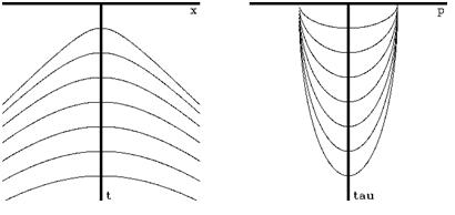Travel-time curves for a data gather on a multilayer earth model of constant velocity before and after slant stacking.

In other words, slant stacking takes us from two dimensions to one, but a  remains to correct the conical wavefront of three dimensions to the plane wave of two.

Stack

A processed seismic record that contains traces that have been added together from different records to reduce noise and improve overall data quality. The number of traces that have been added together during stacking is called the fold.

To sum traces to improve the signal-to-noise ratio, reduce noise and improve seismic data quality. Traces from different shot records with a common reflection point, such as common midpoint (CMP) data, are stacked to form a single trace during seismic processing. Stacking reduces the amount of data by a factor called the fold. 

Velocity

The rate at which a wave travels through a medium (a scalar) or the rate at which a body is displaced in a given direction (a vector), commonly symbolized by v. Unlike the physicist's definition of velocity as a vector, its usage in geophysics is as a property of a medium-distance divided by traveltime. Velocity can be determined from laboratory measurements, acoustic logs, vertical seismic profiles or from velocity analysis of seismic data. Velocity can vary vertically, laterally and azimuthally in anisotropic media such as rocks, and tends to increase with depth in the Earth because compaction reduces porosity. Velocity also varies as a function of how it is derived from the data. For example, the stacking velocity derived from normal moveout measurements of common depth point gathers differs from the average velocity measured vertically from a check-shot or vertical seismic profile (VSP). Velocity would be the same only in a constant velocity (homogeneous) medium. 

NMO Stretching problem(Red) and static problem(blue)

25 % Strech mute

Velocity Analysis  

1Km-V - 2D Supergather- BandPass - Vel Analysis precompute   - Vel Analysis.

First PassOnce flattened, the traces in a NMO-corrected gather can be stacked together for  constructive reinforcement of the reflection events.

Determining the stacking/NMO velocities from the CMG. Here, CMG amplitudes are summed together along different hyperbolas described by the traveltime equation 

t(x) =  

               

V2 =

The summation is carried out for different values of (t0, VNMO), and the result is contoured in (t0,VNMO) space (see the RHS of Figure 1.17). The correct values of (t0, VNMO) will describe an hyperbola that coincides with the reflection event to give a large summation value; otherwise the summation values (or semblance) are small. The summation value is called a semblance value because we really sum over a thick hyperbolic line, weight the summation with a normalization factor, and insure positive summation values by taking the absolute value of the sum. Identifying the bullseyes on the RHS of this figure, and connecting lines between these bullseyes describes the optimal vNMO vs t0curve. The vNMO can also be thought of as the stacking velocity for a layered medium, and is considered to be good estimate of vRMS.

Apparent velocity

The speed of a wavefront in a certain direction, typically measured along a line of receivers and symbolized by v_a. Apparent velocity and velocity are related by the cosine of the angle at which the wavefront approaches the receivers:

Velocity correction

A change made in seismic data to present reflectors realistically. Velocity corrections typically require that assumptions be made about the seismic velocities of the rocks or sediments through which seismic waves pass. 

Stacking velocity

The distance-time relationship determined from analysis of normal moveout (NMO) measurements from common depth point gathers of seismic data. The stacking velocity is used to correct the arrivaltimes of events in the traces for their varying offsets prior to summing, or stacking, the traces to improve the signal-to-noise ratio of the data. 

Interval velocity

The velocity, typically P-wave velocity, of a specific layer or layers of rock, symbolized by v_int and commonly calculated from acoustic logs or from the change in stacking velocity between seismic events on a common midpoint gather. 

Dix

An equation used to calculate the interval velocity within a series of flat, parallel layers, named for American geophysicist C. Hewitt Dix (1905 to 1984). Sheriff (1991) cautions that the equation is misused in situations that do not match Dix's assumptions. The equation is as follows:

Average velocity

In geophysics, the depth divided by the traveltime of a wave to that depth. Average velocity is commonly calculated by assuming a vertical path, parallel layers and straight raypaths, conditions that are quite idealized compared to those actually found in the Earth. 

Wavelet extraction

A step in seismic processing to determine the shape of the wavelet, also known as the embedded wavelet, that would be produced by a wave train impinging upon an interface with a positive reflectioncoefficient. Wavelets may also be extracted by using a model for the reflections in a seismic trace, such as a synthetic seismogram. A wavelet is generated by deconvolving the trace with the set of reflection coefficients of the synthetic seismogram, a process also known as deterministic wavelet extraction. Wavelets may be extracted without a model for the reflections by generating a power spectrum of the data. By making certain assumptions, such as that the power spectrum contains information about the wavelet (and not the geology) and that the wavelet is of a certain phase (minimum, zero), a wavelet may be generated. This is also called statistical wavelet extraction. A particular processing approach to establishing the embedded wavelet is to compare the processed seismic response with the response measured by a vertical seismic profile (VSP) or generated synthetically through a synthetic seismogram in which the embedded wavelet is known. The wavelet can also be extracted through the autocorrelationof the seismic trace, in which case the phase of the wavelet has to be assumed. 

Residual Statics :

Static shifts introduced by topographic variations fall under the class of field statics, and those due to near-surface lithological variations that occur within a cable length fall under the class of residual statics. Correcting for static shifts in the traces can make a significant difference in the quality of a migrated or stacked image. It is easy to determine elevation static corrections, but not so easy to find the residual static corrections. One means is to determine the near-surface velocity distribution by refraction tomography.

It is applied calculating residual shift for consecutive traces in a gather. For a time gate, and respective picked time shift,  it  creates a delta-T matrix and then solves the matrix to give the final output.

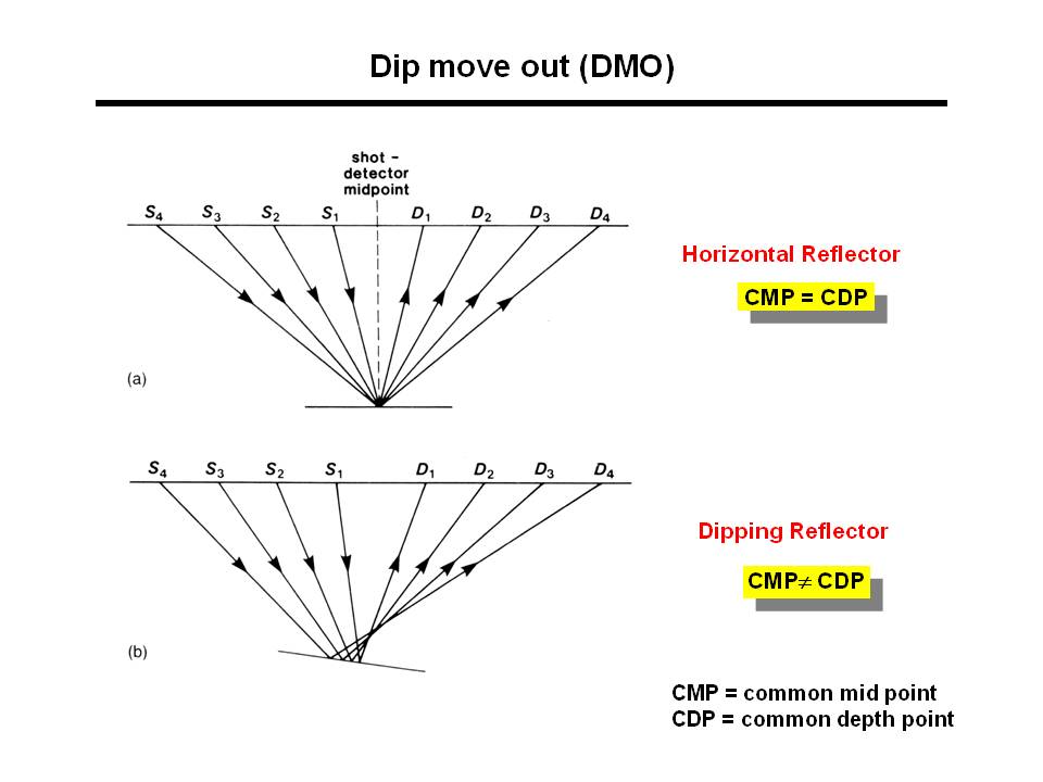
DMO

A seismic processing operation to correct for the fact that, for dipping reflections, the traces of a CMP gather do not involve a common reflection point. DMO effectively corrects for the reflection-point smear that results when reflectors dip. 

Events with various dips stack with the same velocity after DMO.

III IMAGING 

Post-Stack Migrate  MIGRAITON AFTER STACK( After twice Residual static DMO is applied twice to get to raw stack and then DMO pics applied to the raw stack to get final post stack)

Depth Conversion  - VELOCTY MODEL SENSETIVE  - VERY DELICATE TO HANDLE
Pre-Stack Migrate  - EXPENSIVE - MIGRATION BEFORE STACK- VELOCITY ANALYSIS OF GATHERS - Migration is done after Residual Static correction on gathers.

  

Migration

The movement of hydrocarbons from their source into reservoir rocks. The movement of newly generated hydrocarbons out of their source rock is primary migration, also called expulsion. The further movement of the hydrocarbons into reservoir rock in a hydrocarbon trap or other area of accumulation is secondary migration. Migration typically occurs from a structurally low area to a higher area because of the relative buoyancy of hydrocarbons in comparison to the surrounding rock. Migration can be local or can occur along distances of hundreds of kilometers in large sedimentary basins, and is critical to the formation of a viable petroleum system. 

A step in seismic processing in which reflections in seismic data are moved to their correct locations in the x-y-time space of seismic data, including two-way traveltime and position relative to shotpoints. Migration improves seismic interpretation and mapping because the locations of geological structures, especially faults, are more accurate in migrated seismic data. Proper migration collapses diffractions from secondary sources such as reflector terminations against faults and corrects bow ties to form synclines. There are numerous methods of migration, such as dip moveout (DMO), frequency domain, ray-trace and wave-equation migration. 

During seismic processing, migration adjusts the location of events in seismic traces to compensate for dipping reflectors.

Time migration

A migration technique for processing seismic data in areas where lateral velocity changes are not too severe, but structures are complex. Time migration has the effect of moving dipping events on a surface seismic line from apparent locations to their true locations in time. The resulting image is shown in terms of traveltime rather than depth, and must then be converted to depth with an accurate velocity model to be compared to well logs.

Kirchhoff migration

A method of seismic migration that uses the integral form (Kirchhoff equation) of the wave equation. All methods of seismic migration involve the backpropagation (or continuation) of the seismic wavefield from the region where it was measured (Earth's surface or along a borehole) into the region to be imaged. In Kirchhoff migration, this is done by using the Kirchhoff integral representation of a field at a given point as a (weighted) superposition of waves propagating from adjacent points and times. Continuation of the wavefield requires a background model of  seismic velocity, which is usually a model of constant or smoothly varying velocity. Because of the integral form of Kirchhoff migration, its implementation reduces to stacking the data along curves that trace the arrival time of energy scattered by image points in the earth. 

smile

A concave-upward, semicircular event in seismic data that has the appearance of a smile and can be caused by poor data migration or migration of noise.

PSTM:

Prestack Kirchoff Time Migration Dips upto 90 deg. This Algorithm  is applied on common offset non- NMO Corrected gather(through trace binning) , uses both vertically and lateral RMS/stacking velocity from floating datum to final datum(Flat datum).

Maximum Frequency: Less than Nyquist frequency will speed up the computation and above it should be band filtered.

Migration Aperture: Horizontal resolution is twice the vertical resolution so depending upon the depth of interest the apperture test is done to take care of the width of the horizontal distance that energy can migrate.Tapering should be applied. Migration can be split into four conceptual pieces. As a rule of thumb, these four pieces will help us understand what migration is and how it naturally completes the imaging process.

1.The first piece is called normal moveout(NMO). When the world is flat, NMO corrects for the fact that the source and receiver are not coincident, but it cannot do so when the reflections come from dipping horizons.

2.The second piece of migration corrects for dip. Historically, this second piece was called dip-moveout(DMO), but, in the cases of interest here, it happens within the migration methodology itself.

3.The third migration piece shifts events on each moveout-corrected offset to its true subsurface position.

4.The fourth and final piece sums (stacks) all the redundant traces into the final image.

time Migration doesn’t accounts for ray bending, but  interval velocity in depth migration takes care of that.

• Kirchoff
• FK
• Phase Shift
• Finite Difference
• Reverse Time

FX: implemented with spatially variant convolutional filters and are often grouped with finite difference technique12. DAS -Q Compensation - Spectral Whitening - Filter test RADON transforms data to time-moveout space for picking a mute to attenuate energy with undesirable moveout. Radon Filter is commonly used for suppression of multiples. The normal technique is to model multiples and subtract them from the input seismic trace data. Radon filters are then applied to pass the primary energy. However, in practice this tends to produce an artificial and wormy appearing result.